
Finding the minimum spanning tree of an edge-weighted undirected graph is foundational to graph theory. A graphs minimum spanning tree is the collection of edges in an undirected edge-weighted graph that connects all of a graph’s vertices with the minimum overall edge weight. If a graph is disconnected, then the same idea can be expanded to a minimum spanning forest. Algorithms for computing the minimum spanning tree actually predate computers by quite a number of years. Minimum spanning tree’s find use in planning telephone networks, laying out circuit boards, as well as planning roadways, and network routing algorithms. Minimum spanning tree’s , and the algorithms to compute them share much in common with finding shortest paths in a graph, it is worthwhile to understand the differences between them.
There are a number of famous algorithms that have been developed for computing minimum spanning tree’s. Prim’s algorithm – sometimes called Jarnik’s Algorithm – is one such algorithm that was also re-discovered by Edsgar Dijkstra. That essentially the same algorithm was discovered at least 3 separate times speaks to it’s fundamental nature. It is an adaptation of priority first search, and I have covered it in a previous post. In this post I want to discuss what I personally find to be one of the more elegant of the general graph algorithms: Kruskal’s algorithm.
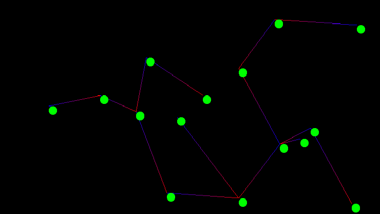
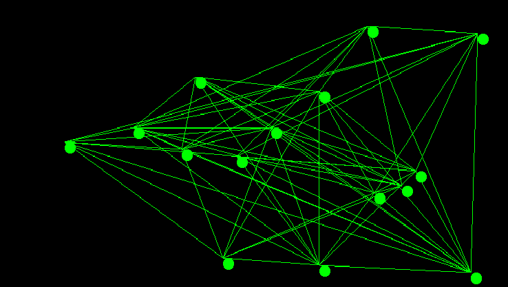
Kruskal’s algorithm is an interesting exercise for computer science students as it leaves many implementation decisions open ended. The outcome of those decisions if not carefully considered can dominate the run time performance of the entire algorithm. The two major design decisions are the choice of sorting method for the graph’s edges, as Kruskal’s algorithm requires the graph’s edges be sorted by edge weight, and the choice of data structure for implementing disjoint sets. In todays post I will go over a particularly elegant implementation that is known to be computationally optimal. The code used in the examples discussed below was also used directly to generate the images of the graph and minimum spanning tree shown above.
Disjoint Sets
There has been alot of research done into the analysis of various disjoint set data structures, and in all reality they deserve a post of their own. For this post I’m going to cover the abridged version. Disjoint sets play a central role in the “union/find” algorithm, which is used for all manner of things, of particular relevance to us, is their use for determining dynamic connectivity. The central idea is that we maintain a list of sets, usually as a parent pointer tree, but I’ve also seen linked versions. This list of sets begins as a list of singleton sets.
Set membership is determined through the use of the equal, merge, and find operations.
class DisjointSet {
     public:
        bool equal(int p, int q);
        int find(int p);
        void merge(int p, int q);
};
There is a very simple way to implement this in just a handful of lines of code. There are also a handful of approaches that make one of either union or find in constant or logarithmic time, these are called quickfind and quickunion respectively. Below is an example of the “simple” approach:
bool equal(int p, int q) {
     return find(p) == find(q);
}
int find(int p) {
   if (p != par[p])
      p = find(u[p]);
   return p;
}
void merge(int p, int q) {
   int proot = find(p);
   int qroot = find(q);
   par[qroot] = proot;
}
While certainly simple, there is a fairly big problem with this implementation. During the merge operation we blindly attach the tree rooted at q to the tree rooted at p, allowing for the potential of the tree to grow incredibly large. Similar to an unbalanced binary search tree, this effects the performance of the find operation, as it now has to traverse longer pointer chains to find the root of a given tree. There are two other methods of similar performance and complexity. “Union by size, with find by path halving” and “Union by rank with path splitting”. Because they are of equivalent performance and complexity, I will only cover the union by size approach, as it’s a little easier to understand. From here on I will refer to this algorithm as “The Union Find(UF) Algorithm”. The UF algorithm allows to perform all operations in logarithmic time. What’s more, its implementation is not much more complicated than the simple version shown above.
The UF algorithm requires two arrays, one for the parent pointer tree, and another to hold the size of the tree rooted at that index. The parent array is initialized with all entries pointing to themselves as their parent, with an associated size of 1. This is our initial set of singletons.
class DisjointSet {
    private:
        int *par;
        int *size;
        int N;
        void makeSet(int i) {
            par[i] = i;
            size[i] = 1;
        }
    public:
        DisjointSet(int numStart = 7) {
            numSets = numStart;
            N = numSets;
            par = new int[N];
            size = new int[N];
            for (int i = 0; i < N; i++) {
                makeSet(i);
            }
        }
        ~DisjointSet() {
            delete [] par;
            delete [] size;
        }
        bool equal(int p, int q) {
            return find(p) == find(q);
        }
Our new implementation of find() make’s use of a technique called “path halving”. Path halving works by traversing the tree and replacing the pointer to the current nodes parent, with a pointer to the current nodes grandparent. This reduces the height of the tree so that the find() operation will complete in logarithmic time.
int find(int p) {
    while (p != par[p]) {
          par[p] = par[par[p]];
          p = par[p];
    }
    return p;
}
The refactored merge() implementation is where we make use of the size array. Previously, we had been merging set’s without regard to the result besides being the same set. In this version, we we merge the sets with the intention of keeping the resultant tree as “flat” as possible. Just like with a binary search tree, the flatter the tree means a shorter the path from/to the root to node, resulting in quicker access times.
void merge(int p, int q) {
     int rp = find(p);
     int rq = find(q);
     if (rp != rq) {
         if (size[rp] < size[rq])
              swap(rp, rq);
         par[rq] = rp;
         size[rp] += size[rq];
     }
}
Now that we have a suitable disjoint set data structure, we can start to tackle Kruskal’s algorithm.
Kruskal’s Algorithm
The high level overview of kruskals algorithm is beautiful for its simplicity. To compute the minimum spanning tree, you begin with a list of the graph’s edges, sorted by weight. From this list of edges, you take the edge with the shortest edge weight and check if adding it to the tree would cause a cycle. If adding the edge to the MST forms a cycle, then it is not part of the MST and can be removed, otherwise leave the edge in place. You proceed this way until you have the V-1 edges that connect the V vertices of the graph with the lowest overall edge weight.
We’re now ready for the next big design decision: how – and to a lesser extent, when – to sort the edges of the graph. No matter whether you have chosen to use an adjacency list or an adjacency matrix as you’re graph representation, we’ve still got some work to do in preparing the edges, as kruskal’s algorithm doesn’t operate directly on either. We need a different kind of graph representation: on edge list. An edge list can be stored explicitly alongside you’re graph as useful metadata, or can be generated “on demand” in a straightforward way from either representation as both store the required information implicitly.
For my Graph data structure I used an adjacency list representation, with the nodes of of the adjacency list being comprised of the following WeightedEdge structure:
struct WeightedEdge {
    int v;
    int u;
    int wt;
    WeightedEdge* next;
    WeightedEdge(int from = 0, int to = 0,int weight = 0) {
        v = from;
        u = to;
        wt = weight;
        next = nullptr;
    }
    bool operator==(const WeightedEdge& we) const {
        return (v == we.v && u == we.u) || (v == we.u && u == we.v);
    }
    bool operator!=(const WeightedEdge& we) const {
        return !(*this==we);
    }
};
I use this edge structure for the adjacency list because it can also be used unmodified for an edge list. This also simplifies things for undirected graphs by not adding back edges to the edge list – something which is much harder to do efficiently when generating the edge list from an adjacency list or matrix. This is stored as an unordered singly linked list so adding an entry can be performed in constant time. The graph structure supplies a public method edges(), which returns an iterator to this list. *For dense graphs this should be avoided, seeing as this problem doesn’t arise when using an adjacency matrix*.
If you’re storing the edge list explicitly, you may be tempted store this list in sorted order. Keep in mind however that this adds an additional O(n) step to every call of addEdge() to the graph – 2 of them, as the graph is undirected. When you consider this would require the algorithm to explore approximately half of the edges in the entire graph – twice – on every insertion, this quickly proves not to be a wise decision. Instead, merge sort is well suited to sorting the list efficiently if the edges are kept in a linked list. Seeing as our edge structure contains a next pointer for use in adjacency lists, it would be silly not to utilize this pointer for the edge list as well. Alternatively, we could store the edge list in an array and use one of any number of O(nlogn) sorting algorithms such as quicksort.
WeightedEdge* Kruskal::merge(WeightedEdge* a, WeightedEdge* b) {
    WeightedEdge d; WeightedEdge* c = &d;
    while (a != nullptr && b != nullptr) {
        if (b->wt > a->wt) {
            c->next = a; a = a->next; c = c->next;
        } else {
            c->next = b; b = b->next; c = c->next;
        }
    }
    c->next = (a == nullptr) ? b:a;
    return d.next;
}

WeightedEdge* Kruskal::mergesort(WeightedEdge* h) {
    if (h == nullptr || h->next == nullptr)
        return h;
    WeightedEdge* fast = h->next->next;
    WeightedEdge* slow = h;
    while (fast != nullptr && fast->next != nullptr) {
        slow = slow->next;
        fast = fast->next->next;
    }
    WeightedEdge* front = h;
    WeightedEdge* back = slow->next;
    slow->next = nullptr;
    return merge(mergesort(front), mergesort(back));
}

WeightedEdge* Kruskal::sortEdges(Graph& G) {
    WeightedEdge* toSort = G.edges().get();
    return mergesort(toSort);
}
As you can se from the above code, the properties of our graph data structure made it well suited to integrating with merge sort. And many real world implementations of kruskal’s algorithm make use of an explicitly sorted edge list. But here’s the rub: If you remember from the graph at the beginning of this post, even a small graph of 15 vertices had 105 edges – with the potential still for much more. At the same time, the minimum spanning tree of any graph has V – 1 edges. That’s a whole lot of sorted edges that we potentially may not end up even needing to examine. What If I told you there was a way we could efficiently get the edges we need for the MST, deferring much of the sorting work until it is needed? There happens to be a data structure which does this extraordinarily well: the min-heap. Instead of explicitly sorting the entire edge list, we will place all of the edges into a priority queue!
struct CompEdge {
        bool operator()(WeightedEdge* lhs, WeightedEdge* rhs) {
            return lhs->wt > rhs->wt;
        }
};

class Kruskal {
    private:
        priority_queue<WeightedEdge*, vector<WeightedEdge*>, CompEdge> pq;
        vector<WeightedEdge*> mstEdges;
        void sortEdges(Graph& G) {
            for (adjIterator it = G.edges(); !it.end(); it = it.next()) {
                pq.push(it.get());
            }
        }
If you’re still wondering how the disjoint set figures into all of this you can relax, as it is union/find’s time to shine. Now that we have access to the list of edges in sorted order, we can use them to greedily build the minimum spanning tree. We use disjoint sets in order to maintain the set of edges that are in the in the MST, from the sets of edges not in the MST in order to determine if adding an edge would form a cycle. This might sound complicated, but its actually the exact kind of problem union/find was designed for! If the two vertices that make up the edge being examined are already in the same set, than adding that edge to the MST would form a cycle. Using this knowledge we can easily determine which edges to add to the MST and which edges we can skip. When we find an edge that belongs in the MST we perform a set union on the sets which contain the vertices that make up that edge in addition to adding the edge to the MST.
As you can see from the code below whether using a priority queue or sorted list, the the algorithm emerges rather naturally:
//Using priority queue
vector<WeightedEdge>& compute(Graph& G) {
    sortEdges(G);
    DisjointSet djs(G.V());
    while (!pq.empty()) {
       int from = pq.top()->v;
       int to = pq.top()->u;
       if (!djs.equal(from, to)) {
            djs.merge(from, to);
            mstEdges.push_back(pq.top());
       }
       pq.pop();
    }
    return mstEdges;
}

//using sorted list
vecotr<WeightedEdge>& compute(Graph& G) {
    DisjointSet djs(G.V());
    for (WeightedEdge* edge = sortEdges(G); edge != nullptr; edge = edge->next) {
        if (!djs.equal(edge->v, edge->u)) {
            djs.merge(edge->v, edge->u);
            mstEdges.push_back(edge);
            if (mstEdges.size() == G.V() - 1) {
                return mstEdges;
            }
        }
    }
    return mstEdges;
}
The above algorithm – both implementations – will compute the minimum spanning tree of a Graph in worst case O(E log E) where E is the number of edges. If you happen to be one of those people who are fascinated by mathematical proofs, Tarjan’s proof of union find using the inverse ackerman function is considered by many to be an excellent example of such.
A quick word on Prim’s algorithm
The other classical algorithm for computing the MST of a graph is Prim’s algorithm. Prim’s will compute the MST in O(E log V), which depending on the density of the graph may be considerably faster than Kruskal’s O(E log E). Like Kruskal’s algorithm, Prim’s algorithm is also a greedy algorithm – though it performs it’s task completely differently. Unlike Kruskal’s algorithm, Prim’s algorithm explores the graph similar to other more “traditional” graph search algorithms like BFS, and Dijkstra’s algorithm in that it uses the Graph’s adjacency API. I also find it to be a less interesting algorithm but that is a purely personal opinion. It certainly is good to have a completely different algorithm to perform the same task so as to be able to compare results from unknown data sets. As such, here is a basic implementation of Prim’s algorithm.
class Prim {
    private:
        priority_queue<pair<int, int>, vector<pair<int,int>>, greater<pair<int,int>>> pq;
        bool *seen;
        int  *cost;
        int  *pred;
        vector<pair<int,int>> _MST;
    public:
        Prim(Graph& G) {
            seen = new bool[G.V()];
            cost = new int[G.V()];
            pred = new int[G.V()];
            for (int i = 0; i < G.V(); i++) {
                seen[i] = false;
                cost[i] = std::numeric_limits<int>::max();
                pred[i] = -1;
            }
            pq.push(make_pair(0, 0));
            while (!pq.empty()) {
                int curr = pq.top().second;
                pq.pop();
                if (!seen[curr]) {
                    seen[curr] = true;
                    if (pred[curr] != -1)
                        _MST.push_back(make_pair(pred[curr], curr));
                    for (auto it = G.adj(curr); !it.end(); it.next()) {
                        if (!seen[it.get()->u] && it.get()->wt < cost[it.get()->u]) {
                            cost[it.get()->u] = it.get()->wt;
                            pq.push(make_pair(cost[it.get()->u], it.get()->u));
                            pred[it.get()->u] = curr;
                        }
                    }
                }
            }
        }
        vector<pair<int,int>>& MST() {
            return _MST;
        }
};
Anyway, that’s all I’ve got for today, If you want the code for todays post, including that for creating the graphics of the MST and Graph, they are available on my Github.
Until next time, Happy Hacking!